2 posts tagged with "LLM"

As large language models (LLMs) continue to grow in size, serving multiple fine-tuned versions of the same base model becomes increasingly challenging. Each specialized version requires significant storage space and memory, making it expensive to deploy many task-specific models. Recent systems like S-LoRA [1] have shown the importance of efficiently serving thousands of model variants concurrently. While parameter-efficient fine-tuning methods like LoRA [2] store only small adapter modules, full fine-tuning and reinforcement learning post-training often update all model parameters, requiring complete model copies for each variant. When you store these fully fine-tuned models for different tasks (say, one for legal documents, another for medical text, and a third for creative writing), each variant requires its own complete checkpoint. For example, an 8B parameter LLM like Llama-3 requires approximately 15GB per variant in FP16 format. If you're serving dozens of such specialized models, the storage and memory costs quickly become prohibitive. Loading and unloading these checkpoints leads to higher latency and cost when providing inference.

However, fine-tuned models aren't actually that different from their base versions. The weight changes introduced during fine-tuning are typically small and structured. Building on compression-based approaches like BitDelta [3], we developed a method that represents weight differences using only their signs (1 bit per weight) plus lightweight scaling factors. The key innovation is using per-axis scaling (either per-row or per-column) rather than a single global scale for the entire weight matrix.

How It Works​

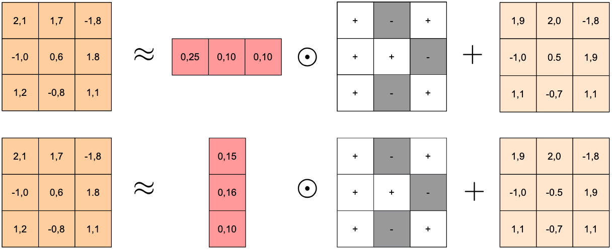
For each layer's weights, we compute the difference between the fine-tuned and base models: $\Delta W = W_{\text{fine-tuned}} - W_{\text{base}}$. We then extract the sign of each weight difference, giving us $B = \text{sign}(\Delta W) \in \{-1, +1\}$. Finally, we learn a vector of scales $\mathbf{v}$ (either one value per row or per column) to reconstruct the fine-tuned weights as $\hat{W} = \mathbf{v} \odot B + W_{\text{base}}$, where $\odot$ represents element-wise multiplication with broadcasting.

The crucial insight is that weight changes during fine-tuning aren't uniform across all dimensions. Some rows or columns of a weight matrix might change significantly, while others barely change at all. A single global scale forces a compromise that either over-scales small changes (adding noise) or under-scales large changes (losing important information). By allowing different scales for different rows or columns, we can better capture these patterns. We automatically select whether to use row or column scaling for each layer based on which reconstructs the model's behavior more accurately.

Rather than trying to match the weights exactly, we focus on preserving what matters: the model's outputs. This follows a similar philosophy to recent quantization methods such as GPTQ [4], which minimize layer-wise output error rather than weight reconstruction error. We use a small calibration dataset (just 50 samples from the C4 dataset [5]) to learn the optimal scales by minimizing the difference between the original fine-tuned model's outputs and our compressed version's outputs: $\mathcal{L} = \frac{1}{n}\|Y - \hat{Y}\|_2^2$. This activation-matching approach ensures that our compressed model behaves similarly to the original, even if the exact weight values differ slightly.

Results and Impact​

We evaluated our method by compressing Llama-3.1-8B-Instruct (the fine-tuned version) relative to Llama-3.1-8B (the base model). Here are the zero-shot accuracy results across five standard benchmarks:

Model	ARC-C	ARC-E	HellaSwag	PIQA	Winogrande	Average
Baseline (Full Model)	51.70	81.81	59.06	79.86	73.87	69.26
BitDelta (scalar)	52.55	82.32	59.73	81.22	73.95	69.95
Our Method (per-axis)	53.58	82.99	59.78	80.63	74.19	70.23

Our per-axis approach achieves the highest average accuracy (70.23%), outperforming both the uncompressed baseline and the scalar BitDelta method, while maintaining roughly the same compression ratio. In our experiments with Llama-3.1-8B, the full FP16 model checkpoint is approximately 15 GB, while our compressed delta needs only 3 GB (a 5.4× reduction). While loading a full fine-tuned Llama-3.1-8B model takes about 2.08 seconds on our machine with RTX4090 GPUs, loading and applying our compressed delta on top of an already-loaded base model takes only 0.80 seconds without any specialized kernels. This makes it much faster to switch between different fine-tuned variants on the fly.

Looking Forward​

Our method works best when the fine-tuning introduces structured changes that vary across dimensions. For layers where changes are more uniform, a simpler scalar approach might suffice. We're exploring several extensions including blockwise scaling for even finer-grained control, learning the sign patterns rather than just using raw signs, and integration with INT4/FP8 quantization for additional compression.

This research supports the infrastructure behind our AI workflow platform at buildbleu.com. When users create and deploy AI backends using our visual workflow builder, we want them to be able to serve multiple specialized model variants efficiently.

References​

[1] Sheng et al., "S-LoRA: Serving Thousands of Concurrent LoRA Adapters", arXiv:2311.03285, 2024

[2] Hu et al., "LoRA: Low-Rank Adaptation of Large Language Models", arXiv:2106.09685, 2021

[3] Liu et al., "BitDelta: Your Fine-Tune May Only Be Worth One Bit", NeurIPS 2024

[4] Frantar et al., "GPTQ: Accurate Post-Training Quantization for Generative Pre-trained Transformers", arXiv:2210.17323, 2023

[5] Raffel et al., "Exploring the Limits of Transfer Learning with a Unified Text-to-Text Transformer", JMLR 2020

Inspired by @karpathy’s talk that LLMs can zero-shot 3Blue1Brown-like videos by writing code in Manim, a Python library designed for creating math animations, we decided to experiment with generating Manim animations with LLMs ourselves. Through a zero-shot approach, we found that while state-of-the-art LLMS are capable of creating short animations (around 15-20 seconds), there were several issues: 1) It is far more difficult for an LLM to generate comprehensible, long-form videos that last several minutes — syntax errors in the Manim code were common, and even if the generated code was error-free, the animation itself was visually unappealing and incomprehensible. 2) A single LLM might take more than 10 minutes to produce Manim code that is free of syntax errors, even though the rendered video would only be 1 minute long. 3) Shorter animations were often visually unappealing as well.

However, with some engineering, we were able to produce higher quality, long-form videos with lower latency. We achieved this through a multi-agent system with an orchestrator agent and several worker agents operating in parallel, RAG on Manim docstrings, and multi-turn prompting (to resolve syntax errors). We’ll explore each of these techniques in greater detail below.

Ku et al. 's TheoremExplainAgent [1] also explores using LLMs to generate long-form videos with Manim and uses similar approaches such as a planner-executor agentic system, RAG, and multi-turn prompting to resolve errors. However, they report that their latency ranges from 18 to 40 minutes. Since we ultimately want users to use our tool, we have an additional latency constraint (less than five minutes).

A Multi-Agent Approach​

Figure 1. Manim AI Workflow

Figure 1 displays our orchestrator-worker agentic system with a planner agent and multiple executor agents. The planner agent generates a scene-by-scene description of the entire video. Then, each executor agent is responsible for generating the Manim code for a single scene. The code is extracted from each executor agent, the scene is rendered, and all scenes are concatenated to produce the final video.

We choose this approach over other approaches for several reasons. First, since we know that LLMs are more robust at generating short videos than long videos, we decide to use this orchestrator-worker approach so that each worker is only responsible for a short video. Second, instead of using a single-threaded linear agentic system, where each worker produces each scene in a sequential order to guarantee that maximum context sharing, we choose an approach in which workers operate in parallel — we sacrifice having agents have full context of the task (different workers don’t have access to each other’s reasoning traces and Manim generations) and therefore robustness [2], but we gain having lower latency due to parallelism. We ensure that each worker agent receives the full conversation history of the planner agent so that the worker has as much context as possible.

Retrieval Augmented Generation (RAG) on Manim Documentation​

For each worker agent, we apply RAG by incorporating relevant sections of the Manim documentation into its context to improve its code generation capabilities. To do this, we parsed and indexed the docstrings from the Manim Github repository [3], and we provide the five most relevant Manim classes to the worker based on the description of the specific scene the worker must generate. We find that this reduces how often the LLM hallucinates Manim function calls and therefore increases the probability that the LLM generates error-free code.

Multi-Turn Prompting​

Since the worker agent may generate Manim code that produces errors during runtime, we apply multi-turn prompting to ensure robustness. Specifically, if the Python runtime produces errors for our LLM-generated code, we add the LLM completion and the Python error to the context of the worker agent and re-prompt it to generate Manim code again. We set the maximum number of attempts to 5; however, we find that with our above strategy the worker agent can often produce error-free code in a single attempt.

Future Work​

Currently, our multi-agent system does not “see” the actual video that it produces. In order to further improve the quality of the video, after the worker agent generates a scene, we would like to provide it with specific frames of a scene as image inputs so that it can improve upon the Manim code if there are visual issues. Additionally, we would like to add community-supported Manim plugins such as manim-physics and manim-chemistry to the context of our system to produce even better visuals.

Finally, Bleu is building an n8n-like tool so that users can produce complex agentic AI workflows with a visual editor. Instead of writing thousands of lines of Python code (as I did for this project), we would like to enable users to produce this Manim generation system simply by dragging and dropping visual components with our workflow, significantly reducing the amount of time it takes to create and deploy AI backends.

Tools used​

We use the Manim Community library for animations and the Manim Voiceover plugin with Elevenlabs to add voiceovers. For code generation, we use Claude Sonnet 4.

Try it out​

Try the Polymath bleuprint to generate math videos with AI.

Citations​

[1] https://arxiv.org/pdf/2502.19400

[2] https://cognition.ai/blog/dont-build-multi-agents

[3] https://github.com/ManimCommunity/manim